Topological Survey Methods with a Total Station

Introduction

In the previous exercise we conducted a distance azimuth exercise, which is a very useful and effective fieldwork technique, but sometimes a higher level of accuracy is necessary or elevation points need to be collected also. In this case, it would be more appropriate to use a total station. A total station is an electronic device used in modern day surveying, it contains an electronic distance meter, and if combined with a GPS unit, location, distance and elevation methods can be taken and recorded. This assignment required us to learn how to set up the station and how to use it alongside the other equipment as, we were to use the open space int he middle of campus to collect data for fifty points using the unit and a sighting pole to make our points. This data could then be uploaded on to a computer and displayed using ArcMap.

The Study Area

The area we were suing to collect our points is know as the campus mall and is about the size of a two hectare plot, the land is a mixture of green space and paving, with a small creek running through it, as a result it lies on a slight slope. Unfortunately I can not show a aerial image of the site, as the last images were taken prior to the area being exposed the way it is today. We were to only study in one hectare plot within this area.

Methods

First of all we started in class by learning to set up the station and the associated tripod. This involved making sure it was set to a height that would be comfortable for our group members to have to be looking through constantly. We then had to attach the unit to the the tripod using the safety screw, and ensure the knobs were pointing away from us to make sure we were going to be bale to take measurements. We had to then look at the spirit level built within the unit, to make sure that the legs of the tripod were all at an equal height, and adjust them accordingly. Then we had t make sure that the unit was level, this was done by turning 3 separate dials on the corners of the unit, with the dial facing towards you, until the display bubble was withing the display circle. An example of a total station unit is shown in figure 1 below.

Figure 1: A total station unit like the one we used during our fieldwork to gather data on point'd distances and elevation. 

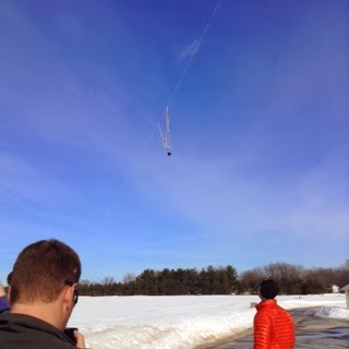
When we were out in the field gathering our data these same processes outlined above were carried out, and is shown in figure 2. We had to use the same azimuth instrument as in the previous exercise to calculate the one hectare plot we would be working in. Then then we had to ensure the Bluetooth was active on the unit in order to sync with the GPS unit to gather the location of points and their associated data. Then the GPS unit, was switched on, the Bluetooth option turned on and we made sure it was synced with the total station. Then on the GPS unit, a new project for our group was created and we selected the appropriate co-ordinate system was selected, we choose NAD 1983 UTM Zone 15N, for the state of Wisconsin. Then we had to enter the height of the sighting pole (in our case 2 meters), the  occupied point which could be read off the display on the total station screen, and the back sight point which we had to collect. This was done by one member of the group selecting and marking with a coloured flag a point and standing there with the total station. Another member of the group then looked through the lens of the total station and lined up the  target on the lens with the center of the upper circle of the sighting pole. Example of sighting poles for use with a total station are shown below in figure 3. The reading of this distance was shown on the station's screen and was entered in to the GPS data.

Figure 2: An image of the total station and tripod put together and being used to find the sighting pole where the photo is taken from.

Figure 3: Examples of sighting poles used in the collection of data with a total station, you can see the black lever which can be sued to adjust the height of the pole, and the central circle on the panel which is used to line up with the station's lens. 

This point is sort of a back up point if you were to have to move your unit. So, the actuall collection of points was done in rather the same matter. Except that now with the GPS linked with the station the measurements would go straight o to the GPS unit. So one member of the group moved around trying to capture the whole scope of the topography of the area as the other lined the station up and waited for the total station to register and transfer the measurements to the GPS units. No flags needed to be placed at these points as we would not need to return to them. For our group we tried to cover the areas in front of and either side of the unit, and go down a bit further in to the creek bank. 

Once we had the desired number of points we were ready to deconstruct our equipment and transfer our data on to the computer. This involved connecting the GPS device to the computer through the use of a GPS cable. The data then appeared as an x,y table on the computer so we had to make sure we added a z field for elevation and the table was imported in to Arc Map and a base ma could be added to give the points some relation. The points could also be taken to create a 3D surface using whichever interpolation technique worked best. 

Discussion

The assignment took a lot of set up and figuring out what to so at the beginning, and we ad run out of time during class to go through every group and show them what to do, so it was quite confusing. The first time we attempted to do it, there were very rainy conditions and the equipment ended up becoming too wet and so we had to abandon our fieldwork. So this could be seen as one disadvantage over the more traditional method which would have still worked during the rain as long as visibility was not impaired. 

When we did mange to complete our fieldwork we had some trouble with the Bluetooth on the total station working as some how it had a code programmed in to it which was not necessary, so we had to seek some assistance with figuring that out and why it wouldn't connect. There were also some points where the GPS would loose connection and quit out of the point recording, but after a while and keeping the GPS as close as possible, this stopped. This would have been easier if we had three people as we were meant to to have one person working the total station, one with the sighting pole and one with the GPS unit.  The person that was holding the sighting pole had to make sure they held it straight upright, so that the station could collect an accurate measurement. The day we did eventually complete our fieldwork the weather was unusually nice and there were many people in the area we were surveying, decreasing slightly the areas we were able to take measurements from. 

In figures 4 and 5 below, we can see to IDW interpolation 3D models that were created from points gathered during the fieldwork, we can see how they contain similarities and differences to each other. It is difficult to explain without having previously been able to show you an image of the study are, but both capture the small creek that was talked about. This is located to the East of the area, my group seemed to capture that valley side to the South, wheres as the other group captured more of the full extent of the creek;s course. Overall the other groups data seems to be more continuous, whereas ours seems slightly edgier, this may be due to the fact that we had so many people in the area that we could not follow a strict sampling method, and perhaps covered some areas better than others. Both capture the general trend of going down in relief as you move further North, with the total station being situated on the area of slightly higher relief. 

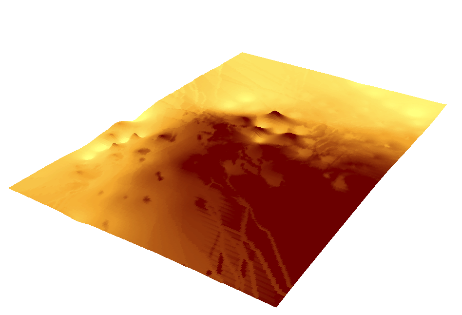
Figure 4: An Inverse Distance Weighted (IDW) Interpolation model of the area my group surveyed. 

Figure 5: An Inverse Distance Weighted (IDW) Interpolation model of another groups data that they collected in the same study area.

Conclusions

Using a total station can collect a wider range of data but takes a lot of set up and good weather conditions. Once you have all the elements set up and the equipment set up, you can gather the points fairly efficiently. But it does rely on the sighting pole being straight and balanced at every point so that all the measurements are comparable to each other.  The results gathered form such a form of data collection will gather different results for different people depending on your sampling method and the conditions you are carrying out the fieldwork in. However, all results should manage to map out the general relief of an area as well as the size and fairly accurately represent the real world phenomena. 

GPS Navigation

Introduction

This exercise was very similar to the traditional navigation exercise and was at the same study area, but this time we were using the more modern navigation strategy of a GPS and completing all 15 points of the full course at the priory. It also required some more work to be done on the maps we produced for navigation to add the points and decide upon a route for our group.There was also the added bonus of the whole class being armed with paintball guns as we were all completing the course!

Methods

First of all we had to go back and edit our maps in ArcMap during class time. Now we had access to the shapefile containing the points of the course as well as the three starting points, so we had to add them and ensure they were a suitable colour to stand out against the background map. Then on this map it was important that we included the polygons for the no-shooting zones, as there was a children's centre in the vicinity and one are was also near a main road, so we did not want to be shooting our paint ball guns in those areas.

Then, as a group we examined the topography and used our knowledge of the five points we had previously found to decided upon a route that would be the easiest to navigate and the fastest to complete. This mainly ensured that if we were going down in relief we stayed down and if we were going up we stayed up, as much as we could. The points shape file's attribute table has the points numbered in the course order, so we had to change this so they were numbered in the order we would be navigating them. Also, the starting points were included int he numbering system, so we made sure they were not included in our numbering system. We also made sure that these numbers were visible so we could see them on the GPS unit screen.

We then attached the GPS unit to the computer with a USB cable, and cut ad pasted a copy of the map file in to the device's folder on the computer. We then turned the unit on and made sure that we could open our map document and that everything that was meant to be displayed was. Also, that there was not to much information on the unit and made the screen to busy so we would not be able to read the map properly. We also had to ensure that we remembered the number of our unit, so we could get the same one when we out in the field so that it had our map file on it.

Whilst out in the field each group had one person with the GPS device navigating the group, as the others were on the lookout for the markers and other groups potentially firing paint balls. The tracklog was switched on, to follow our route and log each time we we had reached a point. We then followed the course displayed , but went of course at times when we had to hide from other groups, so then had to find our way back to the route we were meant to be following.

Discussion

It was quite difficult to decide what to include on the map so as not to overwhelm the GPS unit. We did have to slightly decrease the size of the numbers marking the points,k as they were preventing us from seeing the rest of the map. When using the unit in the field, it was very sort of trial and error, we had to just walk in a direction and see if our track log was following the route or not, and the adjust accordingly until we were following the line on the screen.

There really wasn't much room for us to zoom in or out of the map as it would take a very long time to slowly load, and we were meant to be going as quickly as possible, So, we had already decided that we would print out a copy of our map anyway which came in very handy when the screen would be loading or froze. Our group also did not realise that we had to add a point to the map every time we reached a marker we assumed that it would be shown in the fact that our route had gone past/through the point.

At one point the unit quit out of the map and then took along time to open up again, so we had to seek shelter in a small valley and try and use the paper map without a compass. Then once it had opened again it had lost our tracklog, so according to what our map would show you we did not do the course.

I think that we would have been able to navigate the course a lot quicker if we were using the traditional methods as once we had a rhythm and pattern it worked efficiently. We can also see the whole map and are we need to on a paper map without having to wait to zoom in and out. But I can see how much easier it is to just carry one device, especially when you have paint guns!

Study Area

The study area, as should be apparent, is the same as was used in the previous traditional navigation exercise, except we were physically covering more of the course rather than just one section.

Conclusion

When planning an efficient route it is important to make sure you are not climbing up and down hills constantly, and you do not go back on yourself if possible. When putting a map on to a GPS device you must consider what is necessary to see, so you use as little memory space as possible. As people should do with their Sat-Navs in their cars, you should follow along with map also, so you are not led blindly astray, and you can not always rely on technology to work efficiently and properly. As for the paint balling, I don't really think it was my cup of tea!

Traditional Navigation

Introduction

This exercise was the outcome of the navigation skills and fieldwork map construction we had previously completed, and now that the weather had improved we were bale to put it all in to use. In groups of three we were to navigate a short course of five points using the maps we constructed, a compass and our pace counts we calculated. We had not previously been given the course points and so had to add them to the map in the field and calculate the bearing and distance of each point in order to get to them.

The Study Area

We were completing a course at the Priory in Eau Claire, this is shown in the aerial image in  figure 1.It is an area primarily of forest with varying reliefs with many steep declines to some small creeks. It is off the I94, and about a 15 minute drive from the UW-Eau Claire main campus.

Figure 1: Aerial Image f the priory where the navigation exercise took place. 

Methods

Before setting off on our route we used the co-ordinate grid on the map to mark on the points we needed to go to, then we used a ruler to draw line between these points. A compass was then used to calculate the bearing between points for us to follow during the course. We also used the string of the compass to measure the distance of the lines on the map and then placed that length against the map's scale to calculate the distance between the two points. Within our group we delegate one person to get the bearing on the compass from the map and ensure that we were following it, one person to go to a directed point along the bearing to see g they could see the marker, and the third person was using their pace count to see measure the distance we had traveled to give us an idea if we should be near the marker or not. Once the person looking for the marker had gone to the assigned place, the other two group members followed to then assign a further point that they could see and to check in the t we were headed on the right path. 

Once we had found our marker we then had to use the puncher attached to the marker so stamp the card we had, matching up to the marker number to prove we had found the points. There was no assigned route, but because we were finding points on a section of a course they pretty much followed an order. As there was so much forest around us we could not really use the technique of relating yourself to physical features to find where you are going, but we could use this in the one cleared are we had to go to, you can see i the North East corner of figure 1. 

Discussion

We managed to find all of our points in good time, some of them were a little closer or rather than we originally thought, due to the fact that when you are walking in dense forest you can't really walk in a straight line, moving us in and off course constantly. I think it is worth noting that when we were first getting our bearings they seemed slightly off, but then we realised that it was due to the fact we had been leaning against the bonnet of a car and so the metal was interfering with the magnet of the compass, this also lead to the person using the compass taking off their jewelry so as not to inter fear with it also. 

One of our point we thought was meant to be right in the middle of the clearing and we couldn't see it and we figured that it should be fairly obvious i such an pen are, so we double checked the co-ordinates with where we had placed it on the map and then realised that one of the co-ordinates had been read wrong, so we changed the point on the map and then took bearings from where we knew we were, as we were right on the edge of the forest and could see the road which made it much easier. 

Conclusion

If you have several people working as part of a team you can navigate your way through an area fairly easily, as long as you are all constantly paying attention and ensuring you are sticking to the right path you set. Double checking that points have been plotted correctly before setting off reduces the likelihood of being off course and making sure that you have reduced the compass's exposure to metal is important. Your pace count can vary depending on the type of terrain you are walking on. Being able to see surrounding physical features can help you figure out your position withing an area and on a map. 

The UW-Eau Claire Campus Microclimate

Introduction

This exercise was the second half of the microclimate geodatabase creation for deployment to arc pad exercise. The goals were to go out in to the field and collect micro climate data using a Kestral unit, a compass and a GPS unit, with the hope of creating micro climate maps in ArcMap. From our own groups data as well as the datum collected by the other groups in the class we would be able to get an overall impression of the climatic patterns across our campus.

Study Area

The whole study area was as the title stated the University of Wisconsin- Eau Claire Campus, as shown in figure 1 below. Which comprises of an upper an d lower campus separated by a hill and lies along the Chippewa river. But, the data that my group collected specified in the area just before the hill behind a residence hall and along the river, as can be sen in figure 2.

Figure 1: Aerial Image of the University of Wisconsin-Eau Claire campus, used for a micro climate study. 

Figure 2: The area of the University of Wisconsin- Eau Claire's campus that my group surveyed to collect micro climate data. 

Methods

Our first task was to move the database we had created in the previous exercise to the GPS unit we would be using outside, so that the data points we collected would be recorded correctly and transferred back to the computer easily. In ArcMap we had to make sure that the feature points we collected collected could be seen easily, so we chose a bright pink hue, in order to contrast with the aerial imagery base map we then added to the document. We also had to put the feature classes we previously created in to the map document.

The ArcPad toolbar was found, by selecting the get data button we were walked through the process of deploying our information on t the GPS unit. Once ensuring that our folder was added and the GPS unit was connected to the computer and then our folder was copied and pasted on to the SD card of the unit.

The different climatic factors we were collecting were; temperature, dew point, wind speed, wind direction, relative humidity, the height of the snow and of course the unit was recording our location. The Kestral unit (figure 3) was used for the temperature, dew point, wind speed and relative humidity. A basic field compass was used for the wind direction data collection. A meter stick was also used to record the snow height. The aim was to collect 50 points in our area of campus.

Figure 3: Image of a Kestrel Weather unit, used to take and read measurements of climatic conditions to do with temperature, winds, pressure etc. 

Once we had as many points as the time limit of our class would allow, the data then had to be moved from the GPS unit back in to ArcMap. This was done the same way as the folder was moved on to the unit in the first place, by copying and pasting. All of the groups data then had to be combined in one feature class to examine the whole of campus.

We then had to individually create a series of maps, that would portray different aspects of climate. This was done using ArcMap and techniques used in previous exercises to create maps, and had to be presented including the basic elements of map design. However, we were to put all of the different groups' study areas together so we could have a map for the whole of campus. This involved using the merge tool in ArcMap to put all the feature classes together in one geodatabase, within this coma every groups data was standardised under the parameter's of what the first group used. Some groups were missing descriptions and times in their data, so their part of the columns were left blank but the main data for temperature, wind speed etc, were all filled in.

Discussion

Below in figure 4 you can see all the data points that were collected when you put each group's fieldwork together, it covers on top of and below the hill as well as on and across the footbridge that lies over the Chippewa river.

Figure 4: A map of the points where microclimate data was collected. 

In figure 5 below we can see a map that I created of the wind speed data that was collected. It can be seen that on the day that the fieldwork was carried out wind speeds were fairly calm at round about 3-5mph on average. However there are three noticeable points in the centre of campus that are 9-11mph. This could be due to the fact that these points are between buildings and so the wind would be channeling and concentrated through the space. However the points around it are lower, which would tend to suggest that is not the case and maybe they just picked up a gust of wind in that moment in time. 

Figure 5: Map containing the wind speed in areas of the university campus. 

Some of the measurements may not be as accurate as possible as the readings on the Kestrel were fluctuating so much that we would not have been able to collect all our points if we had waited to get a definitive answer, or it may have not settled on a figure at all. As it was a very cold day, and we perhaps were not quite as appropriately dressed as we should have been, we went inside a building for a few minutes to warm up before continuing. This meant that the sensors were put in to the warmth before going back out in to the cold again and it took some time for them to readjust.

The snow depth and wind direction measurements were perhaps quite controversial also as, the snow depth can var greatly even withing the point you are standing at so it depends very much on where you choose to place the measuring stick.  Some of these areas of snow may also have been there because they were piles of cleared snow, and so would not be accurately representing the real world snow fall measurements. The wind direction was taken from a compass and so was not showing a precise location, but more of a general, direction.

Conclusion

The collection of information of data about an areas microclimate can be fairly simple to collect once you get the use of the equipment and in to a flow. There can be more general readings for points in cases where the Kestrel unit is fluctuating greatly. Physical conditions like snowfall, may have been influenced by man and would not represent the real world phenomenon one hundred percent.

Aerial Mapping through the use of Unmanned Aerial Systems

Introduction

The methods we have been looking in to for taking air images have apart from the kite, so far been highly technological advanced, expensive and still a progressive field. There are some occasions where money will not allow, or the scope of such equipment is simply not necessary, and there for methods like the kite are more suited. So we used a helium balloon to capture images from above ground, in order to be able to mosaic them to ascertain and accurate, detailed, and well presented image of the surveyed land. For the first part we were concentrated on how the fieldwork was carried out, with the idea to spend an extended period of time looking in to and putting in to practice methods of putting together and displaying the images.

 We were also able to go out to the field for a second time with the unmanned aerial vehicle (UAV), as the first time was pretty much a test for the new machine. So now, were were able to witness the drone in it's full flight and the technology and preparation it takes to achieve data collection over a period of time, in order to collect images over a specified area.

Study Area

We used the same study area as was used in the previous exercise where we were introduced to some Unmanned aerial systems,  in Eau Claire's soccer park, because of the open green space.

Methods

The initial equipment set-up was to do with the balloon itself. A large strengthened rubber balloon (obviously significant;y larger and more durable than your every day balloon) was inflated using a helium tank. This was then tied at the bottom and attached to the same spool that we attached to the kite in a previous exercise. The balloon after inflation and before being launched is shown in figure 1.

Figure 1: The  balloon we would be using to gather aerial imagery, post-inflation and before any imaging equipment was attached. 

We then need to attach cameras to the balloon in order to take photos of the terrain. The same "harnessing" device was used as we did for the kite. This involved two digital cameras being attached to stabalisers, and then string to be attached to the cord of the spool on the balloon. Unlike the kite, this did not require a significant amount or height to the balloon first, as it was not going to be diving down to the ground as can happen with a kite. The balloon with the camera harness attached is portrayed in figure 2. 

Figure 2: The balloon in the air with the two digital cameras attached for taking images using a stabalising device. 

We then as a class walked with the balloon around or field site, taking it in turns to hold the balloon and direct, so that we covered the majority of the field site and would acquire multiple images. The balloon was then reeled in and the cameras and stabalisers attached, the SD card from the camera was then used to import the images taken on to a computer system, ready to be used for the mosaic.

The Unmanned Aerial vehicle (shown in figure 3 below) is out of the skill range of the majority of those in the class and so the flight and data collection was very much lead by the class professor, and we were observing and taking notes. We were able to see the laptop (Shown in in figure 4 below) that was used at the control section and it was explained to us how a designated checklist should be made prior to the flight so as to minimise the room for error and make sure everything is working as it should, especially when you are working with such expensive equipment.

Figure 3: The Unmanned Aerial Vehicle at it's starting (and finishing) point before taking flight over the field you can see.

Figure 4: The Laptop set up during the flight of the unmanned aerial vehicle used to observe the flight path to make sure it matches with the pre-set path. 

We learned the importance of looking in to the topography of the area whilst setting up the flight, as the vertical GIS on the device is not great, and you want to  make sure you are going to clear trees etc. On the laptop there is a survey grid so you can follow the path of the device and make sure it is going the same way as the pre-set course. The importance of having two people was emphasised and displayed, so that one person to watch the flight and keep control from the laptop and another to be watching the device int he air and ready with the remote control if necessary. 

As part of the follow up to the fieldwork the class was to look in to and play around with ways of collaborating all the images gathered, so that we could see the whole study area, which is ultimately what you are aiming to do with this sort of fieldwork. We found that Photoscan, a program used by 3D artists and graphic designers, worked well. When adding the images we had to eliminate those that were of poorer quality of were of the cameras initially reaching it's desired elevation, if you were to have taken many more photos over a much larger area then we had, the process of putting them all together could run for a very long time.  The images were then aligned, which created a point cloud, which I have previously talked about in the UAV mission planning assignment.  Building a "Mesh" of these images created a TIN, which we have created from our own data modes before. IN order form images to be georefferenced, we would have to export the TIFF in to ArcMap, then alongside the base map of the are you studied the georeference tool would be used, where you would add control points. Figure 7 below, shown the result that a class member   ( http://fieldmethodreports.blogspot.com/ ) managed to put together form our images. You can see now how we can cover a much wider are. However there are some slight distortions, particularly if we look at the outer parts where it appears more curved. 

Discussion

In figures 5 and 6 below you can see two of the images that were taken using the cameras attached to the balloon. Figure 5 in many ways can be used to compare and contrast with the image that was taken using the kite over the same area, except that this time it is not covered in snow. We ca also see how much higher up in the sky the camera was able to go. Figure 6 shows that with elevated height you can see more of a wider frame, but the slight angle of the photograph does also highlight the problem with using a more basic piece of equipment like the balloon, as the cameras may not stay as stable when attached using the harness and with the effect of the wind. 

Figure 5: The study site from above using the camera attached to the balloon.

Figure 6: The study site and surrounding area from the camera attached to the balloon. 

Figure 7: The images taken from the cameras on the Balloon, put together as a mosaic in the form of a TIFF.

Before we were even able to start the exercise I feel it is worth noting that with such big heavy equipment it required a few people to be able to get the equipment to the field site.  The SD card for one of the cameras was also left out and so once we were all in the field, someone had to go back and retrieve it before we could begin, which in the work force could cost time and money.

When the balloon and camera were being deployed, the camera attachment rope was winding and twisting around the balloon string, so the cameras were less stable, and consequently affecting the quality of those initial images. When we were walking the balloon around the site, the method was not really set before hand, and so the route did not really follow and order. Which will probably result in an unequal covering of areas. 

We were also only able to carry out the survey for about 30 minutes, due to the battery life of the cameras with the system overrides. We were covering a fairly small area, and still felt we needed a little more time t cover it efficiently, so in larger problems this could be problematic. 

The UAV had a similar flight time to the time of the balloon, for battery purposes. It flew very well and matched it's pre-set course and was surprisingly fast when it needed o be and went quite high, it also landed nicely back to where is started from. 

Conclusion

Balloons can be used to take aerial images in a field if money is a factor in a project. The equipment is more basic and easier to use, but may be tricky to transport and handle. Some images may not be very clear due to the effect of the weather on the balloon, this method can not be used in particularly windy unstable conditions. A clear path for taking the balloon over the area you are examining may be needed in order to ensure accuracy and clarity across all areas. The UAV gathers a clearer picture through the use of the stablisers on the vehicle, and can be observed and carried out from a distance and does not require you to physically follow the course yourself, unlike the balloon. But for a much higher price you do get the same amount of time to gather footage. The images you collect can be meshed together using software applications, in order to make use of all the data you created. This can then create an image platform for yuo to perform a number of tasks from. 

Aerial Imaging Equipment Introduction

Introduction

The class took the opportunity from the much improved weather conditions to go outside and test some of the ways of gathering field data we had discussed in the unmanned aerial system mission planning assignment and throughout class . It was simply to see some of the ideas put in to basic practice.

We tested 3 methods of collecting aerial data unmanned with 4 different equipment types. With no specific project set or in mind, other than to capture some images from above where we were, there were no specified attributes to be analysed.

Study Area

We needed an area, that would be fairly clear of people and buildings in order not to invade people's privacy and to have the are beneath clear of people in case the instruments should fall. We used the green area outside Eau Claire's indoor sport's centre and soccer park, as shown in figure 1. It is a flat area covered in grass, with the areas of tarmac for the car park.

Figure 1: Green space in Eau Claire's soccer park used for our aerial imaging. 

Methods

The first method we looked at was unmanned aerial vehicles, where we tested two different types of  remote control rotor copters. Each had on board cameras and GPS devices as well as the operational circuit boards. One had three large  "legs" (figure 2) and another with  smaller "legs"(figure 3). The first one was its first launch, and so when it was flown it was slightly less stable as it calibrated to where it was (figure 4).  The second had been flown many times and so was more stable and was able to get more where it was directed.

Figure 2: The first rotor copter that was used to capture aerial images in the field. 

Figure 3: The second rotor copter that was used to gather aerial images whilst in the field. 

Figure 4: The slightly less stable first rotor copter calibrating on it's first flight. 

We also tried a more basic method of a kite, we assembled the kite (figure 5) then attached the belay device and cast it until it was at about 100 feet (figure 6). A camera was then attached to a form of hamper device and attached to the kite string, and then the kite was cast higher in order for the camera to become high enough to take images. (figure7)

Figure 5: Assembling our kite before flying it to gather data from the air.

Figure 6: The camera once attached to the kite string being sent up in to the air. 

Figure 7: The kite and attached camera high up during data collection. 

The third method we tried was using a rocket with two micro cameras attached to the side. These were very small lightweight cameras as was the rocket, and so were attached to the sides of the craft with industrial tape (figure 8). The rocket was electrically powered and so had a fuse device to set it off with. (figure 9)

Figure 8: Attaching the small cameras to the sides of the rocket. 

Figure 9: The rocket we were using in the field before setting it off, the wire can be seen which lead to the control button. 

Discussion

The rotor copters were by far the most technical advanced, and as such could cover a much wider are much faster, both made use of the emergency device in which the on board G.P.S. unit will direct it back to it's starting position on the ground should control be lost, which I felt was a really good design feature. It also had a device on it that made sure the camera was always in the same steady and stable position which is useful in being able to get high quality comparable images.


If money was an issue in a project or technology, as it so often does fails, then the kite it is a good alternative method. However, it does require the right conditions to be able to fly, and it was relatively quick to set up and deploy.

The rocket launch did not work particularly well for us, and we have yet to see if the cameras were able to catch any stable images which is questionable given the speed of the device.

The results of the photos fro the kite worked well. As it was not positioned extremely high up and we did not walk around with it, only the area directly above us and a little bit around us was covered, but the quality of the picture is good. One of the best images from the days can be seen below in figure10, where the snow covered playing fields, the outbuilding and our group can be seen.

Figure 10: Aerial image taken with the sue of a kite of the area directly above the class.

Conclusion

It was really good to be able to go out in to the field and put in to practice some of the methods that we had spent to long talking about and researching and learning,a little about the technologies and the processes that go in to actually using them. It is good to have a variety of different methods to use in case one does not work, or the project does not dictate that such advanced technology is necessary.

Microclimate Geodatabase Creation for Deployment to ArcPad

Introduction

Data collection in the field should be as efficient as possible in order to make the most of time and money, and still achieve an accurate and satisfactory result. So creating a geodatabase in ArcMap with the fields you will be studying, allows you to out the information you collect straight in to an organised and workable format.

This task was preparing us for some fieldwork data collection we would be doing in order to make a micro climate map of the University of Wisconsin-Eau Claire campus. For us to collect the various datum about the climate we had to create a geodatabase in ArcMap, with feature classes withing that geodatabase that would relate to the various climatic factors we would be measuring. Appropriate domains fo each feature set needed to be stated also.

Methods

When creating a geodatabase for use in the field it is important to consider that there will more than likely be various different attributes  included in the data, each with their own characteristics and unit of measurement. So, one must set pre-defined domains to each different attribute in order to make sure that the data is recorded in a way specified by an employer or project leader and will be within a format that is applicable to that type of data and so can be related to other features.

It also means that results and datum are more easily adjusted, and can be compared with each other and trends noticed and queried whilst in the field. You want the geodatabase to be as easy to use as possible for as many different users as possible s fieldwork can be carried out in groups and data added to the same standards as each other. It allows fieldwork to be undertaken more quickly also. Other users of the ESRI products may also be able to use the data in a way they can understand and edit and add to.

For a climate map such as the one we were to be creating for this geodatabase's use, the attributes that can be recorded include; temperature, wind speed, wind direction, dew point, the relative humidity, snow depth, the time of the data collection as well as any notes on the data that are felt appropriate. Attributed can contain domains with short or whole integers, or float integers. Short and long domains are used for datum whose values contain whole numbers, and float integers are used when those values contain decimal figures.

In order to create our geodatabases  we used the ArcCatalog program, where we directed through the University server to make a folder connection to our own personal class folders. Right clicking on this folder and hovering the cursor over "New..." in the drop down menu, and then selecting "New File Geodatabase", allowed us to create a blank geodatabase.

Clicking twice on this un-named geodatabse slowly, meant we could change the name to something more appropriate e.g. Campus Microclimate. Right clicking on this newly named geodatabase and selecting "Properties..." from the bottom of the drop down menu, opened up the properties window. We then clicked on the "Domain" tab at the top. Here we could add the features we wanted to the table in the window and set the appropriate domains for each.

Clicking on an empty cell in the first column allows you to add a title for a feature, this was repeated for all the desired features. In the second column a description can be given once necessary. When a row is highlighted a second table appears below, and can be used to set the domains. The integer type can be chosen from the drop down menu in the first row, and where a range is necessary for the value this can be typed in to the cell next to the "Range" cell.

For use with the Juno the devices we will be using during our fieldwork a new feature class had to be created. This is done by going back to the "New" option this time in the named database menu and feature class clicked on. Opening the properties of this feature class enabled us to set up the fields in the table in the "Fields" tab, the field was typed in to the rows again and the domains added.

A raster hat had been previously created for the class was imported in tot the geodatabase by right clicking to get the drop down menu, hovering over 'Import...", then selecting the raster file from a folder. Both the feature class and the raster we added to a new map in ArcMap, by dragging them over from ArcCatalgoue, atnd this map was saved ready to input the data post fieldwork.

Conclusions

Creating geodatabses and map documents prior to carrying out fieldwork, can then enable data to be inputted straight to the geodatabse with the use if a handheld digital fieldwork device. Making both the data collection and analysis afterwords more efficient. Data sets can have many different features that require domains to be preset to assure accuracy.

Introduction to Navigation and Fieldwork Map Construction

Introduction

For our next project we shall be navigating our way around a mini orienteering course close to campus without the use of modern day navigation technology like GPS devices.  However, the weather here is Eau Claire is still bitterly cold (there was a wind chill of -3-F today), and there is still much snow on the ground, which would make the task quite challenging at the moment. So we are waiting until conditions improve slightly before carrying out our fieldwork. However, we can still learn about the skills we will need to use in the field in order to be able to find the markers in the field. We explored the more "old school" methods like pacing and compass work, and using the maps to relate yourself to the surrounding physical features what they were and how we could implement them.

We also had to create our own maps for use during our data point collection. This involved employing the computer skills in ArcMap, as well as being able to take in to consideration what elements to include in the map, and he appropriate projection to use for the data. Two maps needed to be produced for a Decimal Degree and Meters data set.

Methods

Pacing is the ability to work out your average number of steps over a certain difference in order to be able to remember this number and use it to calculate how far you have traveled in the field. By knowing the number of steps you usually take to cover a distance, by counting your steps whilst in the field, should be able to work our form the total amount of steps at x steps every x distance, how much ground you have covered.

As a class we went outside to work out our own pace count, so that we could use it in the future. We used the handheld laser distance measures like in the last project to measure out 100m. Then we each walked that 100 meters twice and took the average of how many steps we took each time. MY average was 66 steps, which is around about what most people got, as it's usually between 64 and 68. Except of course if you were particularly tall or particularly short, which would vary dramatically.

The class was then given a quick crash course in compass skills. How to read the values from them and what the different arrows mean were explained. Figure 1 below shows the different elements of a standard compass.

Figure 1: A standard field compass and it's elements ( © paddlinglight.com)

In order to gather where Magnettic North is we turn the compass dial (or bevel) so that the N (North) is in line with the direction of travel arrow. We then standing still move our bodies around until the red arrow is sitting on top of the red arrow drawn inside the compass housing. Calculating a map bearing involves placing the edge of the compass of following the direction of travel arrow point your compass on the map in the direction you are headed. Then adjust the housing until the orientating lines are in line with the latitude and longitude or coordinate systems on the map. The number that is now in line with the direction of travel was before, is the bearing. Bearings are technically given in 3 digit forms, which is fine if your bearing is e.g. 180 degrees, but if it is 20 for example, then we simply put a zero in front, so it becomes 020 degrees.

It is important to use all the information that a map is able to give you when navigating. people that are used to reading maps, especially topographic ones will almost be able to picture the landscape before you even see it. By looking at the contour lines (isobars of elevation) whose interval is usually marked on the map, the water features and having knowledge of how these and other parts of the landscape form can help you to predict what might be happening in the landscape. If pacing is not appropriate then the map scales can be used by utilising the string of your compass, or a nearby branch or something. If you measure a distance on the map, and then hold that up against the scale, you should be able to get the real life value. Sometimes, when a little lost it can help to take a look at significant features on a map and see if  you can identify them in a landscape, and then find your place on the map from there.

In order to make our maps we set up a new geodatabase in ArcMap to save everything to the same place. It was important to ensure that the default geodatabase was set to our own, and that the works pace was pre-set to it also.Then the geodatabase that contained the different shape files, point line and polygon features had to be explored and experimented with in order to decide what would be appropriate for our maps. The sizes and colour schemes of different elements were altered to something that would be easily readable and visually pleasing.

A grid co-ordinate system needed to be added to the maps, as we would be plotting our data points later on out in the field. A different grid system was used for each map from the properties window of the layer, one mad use of meters and the other decimal degrees. This involved also having to select a co-ordinate system for each map. Co-ordinate systems are used to project the earth accurately, as the Earth's shape is actually a geoid and not a sphere as is commonly thought. So, a series of different methods of projecting the Earth on to a flat surface were created, each one however will distort the shape of the earth in some way in; direction, distance, shape, area etc. as it is not possible to deconstruct a round shape on to a flat surface without some degree of distortion. Depending on the area and what you are looking at the system you use will change.

Then some of the essential elements of map design were added using the insert drop down menu. This included; a north arrow, a scale bar and data, projection and co-ordinate system labeling, data sources and our names. AS well as other elements we wanted to include. These were then exported as JPEG images,for use when we carry out our fieldwork. Figures 1 and 2 below show the finished products of the two different maps.

Figure 1: The final map for use in collection of field points using a projected coordinate system that had metres as the units.

Figure 2: The finished map containing a coordinate system that had decimal degrees as its units, for use in data point collection in fieldwork.

Discussion

Pacing is such a basic thing but can be very important and helpful when it is needed. However in areas like thick woodland where there is perhaps lots of vegetation, tree stumps and roots on the ground, you have to take in to consideration that your pace will be a bit slower, It is the same of areas of high relief and in icy or snowy conditions. Also, if this technique is being implemented over a long period of time, then it can be very easy to loose count. A method we were taught to overcome this was to take a twig and every time you reach done of your units of measurement, you would snap it off and put it away fir safe keeping then count all the pieces you have and times that by the distance represented by each.

When deciding upon which map elements to use I added all the different elements at first and decided what was unnecessary as it it did not hold a purpose in helping me in t he field, what image worked better than others in terms of clarity. Also, some elements were obscuring the view of those more important and so were not included.

It is also important not to just stick to a bearing and follow it dead on from the compass, check it against the map and look around often. As we were dealing with the state of Wisconsin and needed something from the UTM zone, I chose the NAD 1983 (2011) UTM Zone 15N, as the projected co-ordinate system, this is one of two UTM zones for Wisconsin, and this is on this covers the area we are studying. NAD 1983 was used for the other map so that the units would be in decimal degrees, and it is a widely excepted coordinate system for U.S. datum.

Conclusions

There are many more skills involved in reading an interpreting a map, than people might have at first thought, It is this bringing together a mix of skills and elements that will make for an effective team in finding points in orienteering. How to use the compass correctly, calculation pace rates, looking at the landscape and identifying on the map, can all help greatly. The projection you use and it's influence needs to be thought about when adding a grid to a map, so as to still remain effective, and not obscure the area too much, which would then make it more difficult to navigate.

Conducting a Distance Azimuth Survey

Introduction

This next field activity was looking in to how data points about an area can be collected more easily than using a co-ordinate system, as was used in the terrain model assignments. We learnt how to make use of some of the older and more recent technology that is available for surveying sights. Our aims were to firstly be introduced to and to try the equipment, then conduct our own group fieldwork. Then, the data needed to be used in ArcMap to produce a map of the data points collected. Throughout the process we were discovering the advantages and disadvantages of different technologies and techniques and some of the problems that people may encounter using these sorts of techniques.

The Study Area

The area we used to practice with the new equipment was located just outside of the academic Science building where our class is held, on the University campus. The area is fairly flat and contains a number of different features with green areas, woodland, car parking space, pavements, lampposts and various signs for the University. Figure 1 below, shows an areal image of the area.


    Figure 1: Aerial image of the first site used to carry out fieldwork. (C. Google Earth)

The study area that my group chose to use for our fieldwork project was located outside of the Nursing building on campus. One of the corners of the building was used as our point of origin, in order to plot our data points on top of an aerial image. The location is similar to the first one and contained trees, poles, signs, mailboxes, bike racks, and some car parking spaces. The land outside of it is a green space and there is a steep slope containing woodland. This are was chosen as due to the high levels of snowfall there had been we needed somewhere local that would be easy to get to and somewhere where all members of the group would be able to meet. We also thought that there would be a good mix of different point types.

Methods
 In class we were introduced to three different types of equipment that can be used to gather information on the distance and azimuth of a point from a source. We then moved outside as a class in order to all have a go at trying each of the methods and to discuss what sort of things we should measure and what should be taken in to account when picking a study site.

One: A filed compass with a built in azimuth viewfinder. Figure 2 below, shows an example of such a device. This is a more basic method that involves less high-tech technology, but is a multistage device. By looking through the viewfinder towards the point you are measuring you can read the scale to collect data on the azimuth of the object from the point of origin.

Figure 2: An example of a field compass with a viewfinder for reading an azimuth recording.

Two: Handheld laser distance measures, this includes two devices, one is held at the starting point and another at the point you are collecting data about and when pointed at one another the distance is recorder digitally on the first device. An example of these devices is displayed in figure 3.

Figure 3: An example of handheld laser distance measures for use in fieldwork.

Three: Trupulse Laser Rangefinder, we found to be the best all round option for ease in the field. This device can be pointed at a recording point and a you can select using buttons on the side what you want to calculate, so both the distance and the azimuth, are displayed and can be read easily and quickly off the screen. An image of what can be seen through the viewfinder and an the device itself is in figure 4 below.

Figure 4: The Trupulse laser rangefinder and what can be seen when looking through it when it's in use.

My group decided that we were going to survey trees, and then decided on our location as discussed previously. A table was constructed before going out in to the field to make the data collection more organised and speedy. Said table with it's filled in value is shown in figure 5. We decided to bring a tripod out with us in order to guarantee, that the origin for the points would be exactly the same, figure 6 is an example of my group collecting and recording data. The attribute we decided to collect was the point type as we felt this would be the quickest and easiest to gather seeing, as we had to wait till late on in the week until everyone in our group could meet to do the fieldwork.  Once we were actually at the site we also saw and decided that we would have to record more features than just trees in order to make up one hundred points. So, once having a look through the viewfinder to see where our maximum range ( 1-4 to 1 hectare plot), and then selected points to measure and the point number, attribute type, distance from origin (m) and azimuth from origin (Degrees) were collected.

Figure 5: The table that our group used post data collection in the field.

Figure 6: Two members of my group collecting data using the Trupulse and recording it into a spreadsheet.


This table was then converted into digital form by typing the values into a excel spreadsheet, A base map satellite image of the field area was added to a blank map in Arc GIS (figure 7), and then using the same corner that we measured from on the nursing building we were able to read of the bottom of the screen the origin x and y co-ordinates, by holding the cursor over it. The x and y co-ordinates were then added to each data poin in the table, in order to be able to export the table to Arc Map.

Figure 7: The base map used in ArcMap to display recorded points on.

A geodatabase was set up in Arc Map and then the excel table was imported in to it. ArcToolbox was opened, then we went in to Data Management, Features and double clicked Bearing Distance to Line. A window then opened up where we had to select or data table as the input and select the various fields, then the lines were added to the map to show the distance and azimuth from our starting point, as conveyed in figure 8.

Figure 8: The AcrMap basemap once the Bearing Distance to Line tool had been applied.

We wanted to have our data displayed as points also, to in the same features toolbox the Feature Vertices to Points command was used, and the same process as before was applied. Figure 9 now shows the final map created from our fieldwork.

Figure 9: Final Map of the distance azimuth survey on campus. 

Discussion

As mentioned slightly in the methods section, as a class we decided that the Trupulse laser rangefinder was the best for carrying out our fieldwork. As, it is able to carry out a greater number of measurements the other pieces of equipment, the data is displayed for you so you do not have to read it off a scale, and if you were by yourself you could carry out fieldwork alone fairly easily.

When we arrived at our site we were able to see just how much of our view was obstructed by the buildings and how many data points would be within our distance range, and it did not look like enough, so it meant we had ti branch out to different types of points. But I think it gives a better impression of what is actually at the location. Also, with the trees it was quite difficult to tell them apart at this time of year, as they were closely situated next to each other, had shed their leaves and were covered in snow.

Towards the end of our data collection there was some precipitation starting to fall which was obstructing the lens, so we had to make sure that was clear. Entering the data in to excel was fairly time consuming and can be quite frustrating when you already have it in a table from and it's just not digitised. So we have decided that during future field work, (weather permitting) we shall use my iPad to record the data on, so that it goes straight in to a digital form and can save some time.

The first few times that the Bearing Distance to Line feature was used it failed, as some of the table categories and names contained numbers and punctuation which did not allow the tool to run, so this had to be altered. Bright colours had to be used for the line and point displays in order to be visible against the satellite image.

This technique for collecting field data is very useful as it is much easier to be able to stay in the same location with all your equipment and record data than having to go out to each point, especially if you were doing this on a larger scale. It is time effective, and as previously mentioned is suitable if you were carrying out a project alone. It can be used for nay form of data collection where you need to measure how far away points are from each other, their distribution, the prevalence of something occurring. It can in many cases be used in conjunction with GIS or in fact replaced with GIS if no fieldwork were to be involved.

The gathering, recording and displaying of data seemed to all go well, and so I feel that our results are probably fairly accurate. Especially seeing as we made use of a tripod, it meant that we could ensure that all the measurements originated in exactly the same location. Of course there is always the chance that technology will fail you and perhaps won't be completely accurate, or that they may be read or recorded wrong.

Also, with Azimuth calculations there is always the problem of magnetic declination, this is the angle between North and true North. This varies according to location and changes over time. Using the National Oceanic and Atmosphere Administration website, you can calculate the magnetic variation for your site, the calculation for our groups fieldwork site is shown in figure 10.

Figure 10: The NOAA calculation of the magnetic declination for our azimuth survey fieldwork location.

Conclusions

There are many different methods and instruments that can be used nowadays to measure the distance and azimuth of selected features whilst carrying out fieldwork, one that can calculate a wide variety of measurements quickly and easily is preferable. it is important when collecting points from a source, that the source remains the same each time, and magnetic declination must be taken in to account when calculating the azimuth. Tables being used in ArcMap must have simple headings and titles in order for tools to run successfully. The type of data that you can collect whilst doing fieldwork can alter when you see the site for real than when you look at it on a map or are planning, and some things may be more difficult o see or measure depending on the weather conditions.